Handling Dynamic Shapes

This document uses “dynamic shapes” as a broad term describing model behaviors where certain topologies generate variable output tensor shapes due to dynamic input data or operators. This dynamicity may cause constant re-compilations, leading to longer training time.

The following sections discuss methods to detect dynamic shapes and mitigate their impact on model performance.

Types of Dynamicity

Dynamic shapes can be broadly classified into two categories:

• Inputs - Dynamic shapes due to varying input shapes during training, such as:

  • Varying sentence lengths in language models

  • Differing image resolutions in image model

• Ops - Dynamic shapes due to ops where the output shape depends on the specific input data, rather than just the input shapes, such as ops with non-inferable output shapes based solely on input shapes.

Detecting and Mitigating Dynamicity Overview

Dynamicity, resulting from changing input shapes or dynamic ops, can lead to multiple recompilations, causing a longer training time and reducing performance. Below are the guidelines to detect and mitigate this issue:

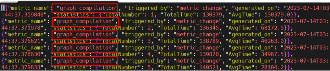
1. Detecting model recompilation - To detect if the model is recompiling, set the following environment flags: PT_HPU_METRICS_FILE=/root/metricslog.json, PT_HPU_METRICS_DUMP_TRIGGERS=process_exit,metric_change. The image below displays the text graph_compilation, which is dumped into the specified JSON file every time a compilation occurs. For static graphs, a reduction in recompilations is expected after a few steps. If recompilations continue to occur after adding the above flags, go to step 2.

2. Enabling dynamicity support from graph compiler - To enable dynamicity support, set the PT_HPU_ENABLE_REFINE_DYNAMIC_SHAPES=1 flag, as it is disabled by default. For further details, refer to Graph Compiler Dynamicity Support. If recompilations occur, or you encounter instability and want to achieve better performance, go to step 3 and 4.

3. Detecting dynamic shapes due to varying inputs - Use the data_dynamicity tool to generate a report on input dynamicity as described in Detecting Dynamic Inputs. If there is a large amount of variability in the input data, use data bucketing and padding as described in Mitigation Through Bucketing and Padding.

4. Detecting dynamic shapes due to ops - Use the detect_recompilation_auto_model tool to automatically detect which part of the model has dynamic ops as described in Detecting Dynamic Ops. If the model has dynamic ops, replace the dynamic ops with static ops as described in Replacing Dynamic Ops with Static Ops. If replacing dynamic ops with static ops is not possible, split dynamic and static sections to make recompiling section smaller as described in Splitting Dynamic and Static Sections.

5. If you are running steps 2-4 in a multi-card scenario, enable recipe caching via PT_HPU_RECIPE_CACHE_CONFIG. For more details, refer to Runtime Environment Variables. This allows one card to use the previously compiled graphs from another card.

Graph Compiler Dynamicity Support

To enable dynamicity support, set the PT_HPU_ENABLE_REFINE_DYNAMIC_SHAPES=1, as it is disabled by default. If a model experiences excessive recompilations due to dynamic data or ops, this variable can be set to enable the Intel Gaudi PyTorch bridge and graph compiler to automatically manage dynamic shapes in model scripts. The graphs will be automatically bucketed and padded into ranges to achieve a common size, reducing recompilations and improving performance when working with dynamic workloads.

In a multi-card scenario, enable recipe caching via PT_HPU_RECIPE_CACHE_CONFIG. For more details, refer to Runtime Environment Variables. This allows one card to use previously compiled graphs from another card. If recompilations continue to exist, or you encounter instability, refer to the following sections to detect dynamicity and find tips on rewriting the model.

Dynamic Shapes due to Varying Inputs

Detecting Dynamic Inputs

The data_dynamicity tool detects the distribution of the input data’s shapes and generates a report on input dynamicity. The below examples demonstrate the tool usage.

• MNIST dataset:

  from habana_frameworks.torch.utils.experimental import data_dynamicity
  import torchvision
  from torch.utils.data import DataLoader
  
  # Creating a sample MNIST dataloader
  mnist_ds = torchvision.datasets.MNIST('mnist', download=True, transform=torchvision.transforms.ToTensor())
  mnist_dl = DataLoader(mnist_ds, batch_size=7, num_workers=2)
  
  data_dynamicity(mnist_dl)
  

  Expected output:

  

  The MNIST dataset has a constant image shape, but two distinct input shapes are obtained, since the last batch has less number of images if there is no drop_last=True (in mnist_dl = DataLoader). In this case input dynamicity is low, so no changes are required for the input.

• Food101 dataset:

  from habana_frameworks.torch.utils.experimental import data_dynamicity
  import torchvision
  from torch.utils.data import DataLoader
  import torch
  
  
  def collate(batch):
     dim1 = min([k[0].shape[1] for k in batch])
     dim2 = min([k[0].shape[2] for k in batch])
     images = torch.stack([k[0][:,:dim1,:dim2] for k in batch])
     labels = torch.tensor([k[1] for k in batch])
     return (images,labels)
  
  food101_ds = torchvision.datasets.Food101('food101', download=True, transform=torchvision.transforms.ToTensor())
  food101_dl = DataLoader(food101_ds, batch_size=7, num_workers=2, collate_fn=collate)
  data_dynamicity(food101_dl)
  

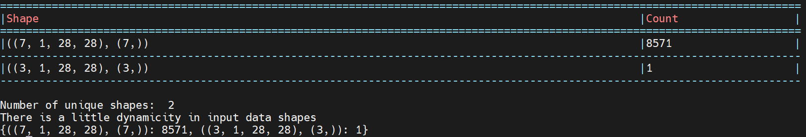
  This dataset contains images of different shapes. In the example above, batches are created by cropping the images to the size of the smallest image in each batch.

  A large amount of input dynamicity is obtained for Food101:

  Number of unique shapes:  66
  # There is a lot of dynamicity in input data shapes
  

  If there is a large amount of variability in the input data, data padding and/or data bucketing can be used. Refer to the section below.

Mitigation Through Bucketing and Padding

Bucketing and padding can reduce the number of unique shapes in input data. The input data shapes are divided into buckets of varying sizes, and data points are padded up to the smallest bucket larger than the largest data in each batch. In bucketing algorithms, the number of buckets is a hyperparameter. Choosing a large number of buckets causes many recompilations, while choosing a low number of buckets requires excessive padding and, therefore, causes unnecessary computations.

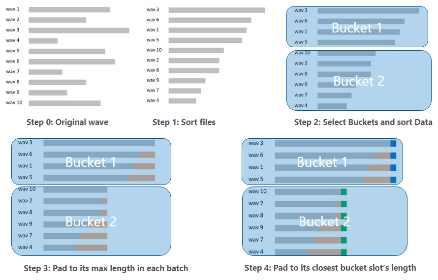
The example below shows how to take a random dataset of wav files, create two buckets and then sort and pad the data.

Bucketing algorithms can be classified into two categories. You can use any novel padding/bucketing strategy to get the best tradeoff between bucketing algorithm time, compilation delays and HPU runtime speeds. The following table lists the suggested bucketing algorithms:

Bucketing Algorithm Type	Description
Optimization-based	These algorithms have a criterion function to optimize. For example, the linear programming approach to reduce amount of padding wastage is used in fairseq. Usually these methods are slower, but are more optimal when using less padding.
Fast heuristics-based	These bucketing algorithms are quick and easy to use. However, these methods usually have more padding wastage than the optimization-based methods. percentile-based bucketing, which is also discussed in the Case Study Using Wav2vec2 for Dynamic Inputs to Models. Constant width bucketing where each bucket is of constant width between minimum and maximum data length. Padding to max length.

Preprocessing Input Dataset

When the input dataset is large, processing all the shapes in it, especially for costlier optimization based bucketing algorithms, might be too slow. To bypass this issue, perform the following:

• Shuffle the shapes of the dataset and pick a small number of shapes to pass to the bucketing algorithm, reducing its workload.

• Rather than creating a histogram for each shape, create a histogram with a wider bin, so that multiple contiguous shapes fall in the same bin.

Saving Bucketing Results

If the bucketing algorithm takes a lot of time, computing it every time you run the script is inefficient. You can store the results of the bucketing algorithm based on the hash of the input shapes. For example, see here. For example:

import hashlib
lst = [2, 4, 5, 3, 6, 3, 2]
key = hashlib.sha256(bytes(sorted(lst))).hexdigest().upper()

Variable Batch Size

You can adjust the batch size using bucketing. When using a fixed batch size, shorter input data may not fully utilize the device because a larger batch size could have been accommodated. If the batch size is too large, it might lead to Out of Memory errors when processing larger input data. Thus, it is advisable to use a larger batch size for shorter sequences and vice versa: batch_size=max_num_words/sentence_length.

Refer to Memory Stats APIs for more information on memory usage.

Note

When there is a possibility of dynamic shapes distribution, running bucketing is beneficial. Some examples of multiple distributions are:

• Multiple inputs - A model might have two inputs, each with its own dynamic distribution of input shapes. Running bucketing separately on both inputs is recommended. An example of such a scenario is translation task, where the source and target language sentences might have different distributions.

• Multiple datasets - If you use multiple datasets, running bucketing algorithm for each dataset separately is recommended. For example, Roboflow is made of 100 different datasets, all training on the same model in 100 different runs.

Dynamic Shapes due to Ops

For certain ops, such as the following, the output shape cannot be predicted, even if the input shape is known:

• Unique

• Single input Where (identical to Nonzero)

• Nonzero

• Boolean indexing

Detecting Dynamic Ops

To detect dynamic ops, perform a simple string search in the repo for ops or run the script with GRAPH_VISUALIZATION=1 to create a .graph_dumps folder and monitor it to see if the number of graphs dumped keeps increasing. If dynamic shapes are present, multiple recompilations cause the number of dumps in the .graph_dumps folder to increase.

Note

To detect dynamic ops, make sure to use same sized inputs to avoid recompilations due to varying input shapes.

To find out which part of the model has dynamic ops, use the detect_recompilation_auto_model tool. The code snippet below shows inference on a model with a dynamic op (boolean indexing) and dynamic inputs (changing batch size):

from habana_frameworks.torch.utils.experimental import detect_recompilation_auto_model
import torch

class InnerNet(torch.nn.Module):
   def __init__(self):
      super(InnerNet, self).__init__()
      self.conv = torch.nn.Conv2d(1, 8, 3, 3)

   def forward(self, x):
      x = torch.flatten(self.conv(x), 1)
      x = x[x>0] # This is dynamic
      return x.sum()

net = torch.nn.Sequential(torch.nn.ReLU(), InnerNet())
net = detect_recompilation_auto_model(net)

for bs in [20,20,20,30,30]: #Input shape changes at 4th step
   inp = torch.rand(bs, 1, 50, 50).to('hpu')
   print(net(inp))
net.analyse_dynamicity() # Call this after a few steps to generate the dynamicity report

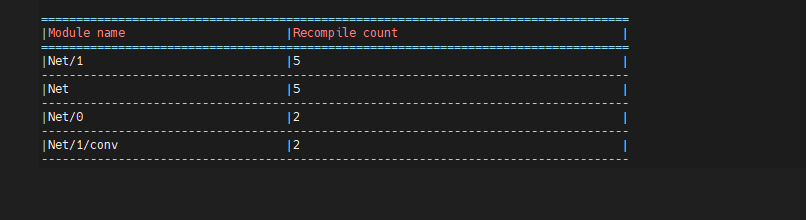
This produces the following report (along with the CSV versions of it):

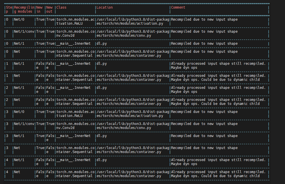
0. The first four lines of the first table show all four modules recompile since it is the initial step.

1. The next two lines show Net and InnerNet recompile. The “Comment” column, however, shows that InnerNet might be dynamic because it recompiled even without dynamic children modules. Net may not be dynamic as it might have recompiled because its child (InnerNet) has recompiled.

2. The next two lines show step 2 which is similar to step 1.

3. The next four lines show step 3, where a new input shape is seen, so every module recompiles as expected shown in the “Comment” column.

4. The last two lines for step 4 point to InnerNet as having dynamic ops.

The table below is a summarized view that shows which modules recompile the most. As expected, Net/1 of type InnerNet (and its parent) show up at the top.

Note

The detect_recompilation_auto_model tool slows down model execution, so it is only intended for debugging purposes and should be removed for the actual run.

Mitigation Techniques for Dynamic Ops

Replacing Dynamic Ops with Static Ops

Removing dynamicity needs a case-by-case inspection but the general guideline is to identify the section of the code where dynamicity starts and ends, then replace it with static code. See the below examples.

• Example 1 - This example of boolean indexing which is dynamic can be replaced to make the code static:

  #Dynamic code
  
  non_pad_mask = targets.ne(self.padding_idx).view(-1)
  smooth_loss = smooth_loss[non_pad_mask]
  smooth_loss = smooth_loss.sum()
  
  #Static Code
  
  non_pad_mask = targets.ne(self.padding_idx).view(-1)
  smooth_loss = smooth_loss.squeeze() * non_pad_mask.int()
  smooth_loss = smooth_loss.sum()
  

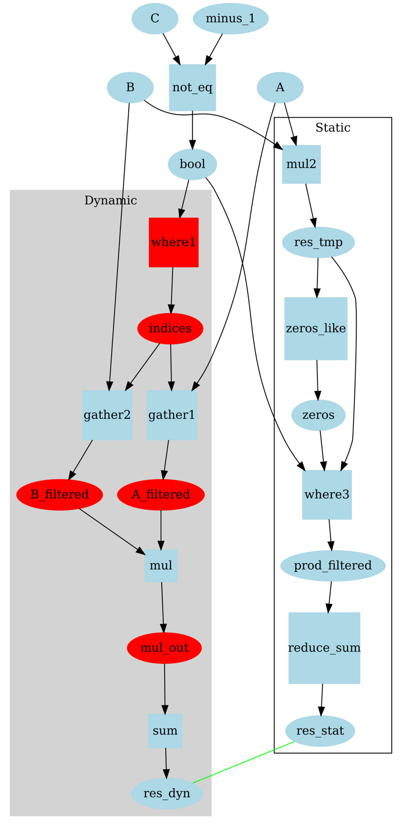
• Example 2 - If a tensor A, B, and C of length N is given, with C[i] being –1, the corresponding elements are filtered out. The remaining elements are then multiplied A[i]*B[i], and the results are added up.

  Pseudocode: res = sum([A[i]*B[i] for i in range(len(C)) if C[i] != -1]).

  #Dynamic code
  
  import torch
  import habana_frameworks.torch.core as htcore
  
  A = torch.tensor([1,2,3,4,5]).to('hpu')
  B = torch.tensor([6,7,8,9,10]).to('hpu')
  C = torch.tensor([1,-1,1,1,-1]).to('hpu')
  
  indices=torch.where(C!=-1)
  A_filtered=torch.gather(A, 0, indices[0])
  B_filtered=torch.gather(B, 0, indices[0])
  
  res_dyn = torch.sum(A_filtered * B_filtered)
  
  #Static Code
  
  res_tmp = A*B
  prod_filtererd = torch.where(C!=-1, res_tmp, torch.zeros_like(res_tmp))
  res_stat = torch.sum(prod_filtererd)
  
  assert (res_stat == res_dyn).item()
  

  In this example we identify the start of dynamicity (where) and its end (sum) and replace it with a static implementation. The diagram below shows the two possible paths, with the dynamic nodes and tensors marked in red.

Explicit CPU Fallback

In normal mode, ops that are not supported on HPU are already automatically placed on the CPU as explained in Placement of Ops on HPU. Explicit CPU fallback refers to moving certain ops to the CPU (and possibly later bringing them back on the HPU) explicitly for dynamic ops. For example:

#say x is on HPU
z = torch.unique(x) #this op is done on HPU because input x is on HPU
# can be replaced by:
x=x.to('cpu')
z = torch.unique(x) # runs on cpu
#move tensors back to HPU if needed
x = x.to('hpu')
z = z.to('hpu')

Sections on the CPU can be sped up using torch jit by wrapping them in the @torch.jit.script decorator.

Splitting Dynamic and Static Sections

Consider a case where the network starts with static layers, has a few dynamic layers, and then ends with static layers. Under normal circumstances, the whole network recompiles in each step, making execution slow. However, we can add mark_step between the static and dynamic sections of the network. With this change, the static part compiles only once, and the dynamic part is smaller (compared to the whole network) and hence compiles faster.

# The whole network static1->dynamic->static2 recompiles
x = static1(x)
x = dynamic(x)
x = static2(x)

# After splitting them, now only dynamic recompiles. static1 and static2 compile only once
x = static1(x)
mark_step()
x = dynamic(x)
mark_step()
x = static2(x)

Note

When possible, replacing dynamic code with static code, as detailed in Replacing Dynamic Ops with Static Ops, is recommended. If it cannot be done, try CPU fallback or splitting dynamic and static ops or do not make any change to figure out which option is fastest. Depending on the model, each method has its own advantages and disadvantages. CPU fallback might trigger costly host-to-device or device-to-host copies. While splitting reduces the compile time, there is still dynamicity and hence compilations happen.

Dynamic Shapes in Distributed Training

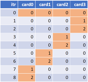
If we have S shapes and N cards, in the worst case scenario, N*(S-1) + 1 compilation delays is observed. This means only one card is compiling a new shape, while the other cards receive shapes they have compiled before. Those cards finish compiling faster and remain idle. The figures below show the inefficiency of cards having to sit idle while waiting to compile new shapes (highlighted).

To mitigate this issue, use across rank caching. When a new shape is encountered, its recipe is saved to file, allowing other cards to use it instead of recompiling each new shape. To do this, set the below:

PT_HPU_RECIPE_CACHE_CONFIG=/tmp/iter1_recipe_cache/,true,1024

Case Study Using Wav2vec2 for Dynamic Inputs to Models

Models with dynamic input shapes are constantly recompiled resulting in longer training time. In audio models, it is common that the input contains wave files with variant length. The steps below outline the bucketing and padding solution steps required to achieve better training performance on Gaudi using Wav2vec2 as an example.

Bucketing and Padding Solution Example

1. Sort the wave files according to the length. This is to make sure that wave files with similar length are grouped together to decrease possible padding.

2. Define the size of buckets. According to the distribution of wave file length in the dataset and the number of bucket slots the user defined, define the length of each bucket slot. A general rule in Wave2vec is to define the length of a bucket so that the number of files falling into different buckets are similar.

   Below is the example code that Wav2vec uses to define the length of different bucket via numpys percentile function, where sizes is an array that contains the size of all wave files and num_buckets is the number of buckets you want to use:

   def get_buckets(sizes, num_buckets):
      buckets = np.unique(
         np.percentile(
               sizes,
               np.linspace(0, 100, num_buckets + 1),
               interpolation="lower",
         )[1:]
      )
      return buckets
   

3. Split the dataset into different batches. For example, in Wav2vec, a threshold value is defined to make sure the total file size in one batch does not exceed this threshold value. Refer to the example here.

4. Padding:

   1. Pad wave files in the same batch to the same file size. To make sure each wave file in the same batch has the same size, it is padded to the max file size in that batch.

   2. Pad wave files in the same batch to the bucket size. When the file length in the batch is not the same as the bucket length, it needs to be padded to match the length of the bucket with the closest distance. This way, even if there are a lot of batches, the shape of those batches will be limited.

   You can find a padding example using Wav2vec2 here.

With this bucketing and padding solution, the number of dynamic shapes of the input to Wav2vec can be greatly decreased. Refer to the implementation in Wav2vec2 Model Reference on GitHub.