HPU Graphs for Training
On this Page
HPU Graphs for Training
Lazy mode, supported on PyTorch, accumulates and flushes ops only when mark_step is triggered.
In large models, the accumulation time for the ops (host time) can be significantly greater than for
devices. This could decrease the model’s performance by making it host-bound.
HPU Graphs feature overcomes this bottleneck by bypassing all the op accumulations by recording a static version of the entire graph, and then replaying it. These static graphs use fixed memory locations for its inputs, outputs, and the underlying graph. While HPU Graphs reduce host overhead significantly, dynamic flexibility of the model is compromised.
HPU Graph APIs are similar to the CUDA graph APIs, but they provide extra wrappers such as ModuleCacher.
Note
Running HPU Graphs is supported with Lazy mode. Eager mode is currently not supported.
Theory of Operations
When training a model without HPU Graphs, ops are accumulated to create a graph and compile a recipe. For each iteration, the entire graph is parsed. HPU Graphs speeds up this process as subsequent iterations check the input shapes only. HPU Graphs assumes there is no dynamic op or dynamic flow in the graph, and relies on input shapes only to determine whether the precompiled recipe can be used or if a recompilation is required.
Note
HPU Graphs should be used for static ops. Data-dependent dynamic flow is not supported. For example:
Data-dependent
if-elsestatements in Python code.Data-dependent
fororwhileloops in Python code.Dynamic ops whose output sizes depend on input sizes. See Dynamic Shapes due to Ops.
Using HPU Graph APIs
In addition to HPU Graph basic APIs, such as capture and replay,
Intel Gaudi also provides graph, make_graphed_callables and ModuleCacher APIs for your training model.
The purpose of these APIs is to make your code more streamlined.
Unlike the basic HPU Graph APIs, ModuleCacher API accepts non-tensor and non-positional arguments.
For more details, see Simple MNIST Example with HPU Graph APIs.
While only static graphs are supported, separate graphs are compiled for different-shaped inputs or for different paths
of the dynamic control flow with ModuleCacher API. Therefore, it can be used for training models with dynamic inputs. For more details, see Dynamicity in Models.
HPU Graph APIs Overview
The following section describes the usage of basic and high level HPU Graph APIs in a training model. For a detailed description of each API, refer to HPU Graph APIs.
capture_begin, capture_end, and replay() - These APIs are similar to the CUDA capture and replay APIs. The following example shows how to replace
cuda.CUDAGraph.capture_beginwithhpu.HPUGraph.capture_begin:#torch.cuda.CUDAGraph.capture_begin() import habana_frameworks.torch.core as htcore htcore.hpu.HPUGraph.capture_begin()
graph and make_graphed_callables - These APIs are similar to the CUDA graph API and CUDA
make_graphed_callablesAPI. The following example shows how to replacecuda.make_graphed_callableswithhpu.make_graphed_callables:#torch.cuda.make_graphed_callables(...) import habana_frameworks.torch.core as htcore htcore.hpu.make_graphed_callables(...)
ModuleCacher - This API provides another way of wrapping the model and handles dynamic inputs.
ModuleCacherinternally keeps track of whether an input shape has changed, and if so, creates a new HPU graph. It also enables accepting non-tensor and non-positional arguments which is a limitation when using the basic HPU Graph APIs. See Limitations of HPU Graph APIs.model = Net().to('hpu') htcore.hpu.ModuleCacher(max_graphs=10)(model=model, inplace=True)
Note
The basic APIs are useful in static graphs with no dynamic control. Also, the models can only input tensors and positional arguments.
Run a host profile to make sure the model is host-bound. If it is device-bound, using HPU Graphs is not beneficial.
For dynamic inputs, use
ModuleCacher. This API also provides a workaround for the input limitation where only tensors and positional arguments are supported.ModuleCacherdoes not handle dynamic control flow or dynamic ops.Make sure to set sync/mark_step. For further details on
mark_step, refer to mark_step section.Even simple models with static inputs might exhibit dynamicity. For example, if the batch size does not divide the dataset evenly, one gets a batch at the end that is a different shape than the ones that came before it. This can handled by using
ModuleCacheror by usingdrop_last=Truein the dataloader.Inference is also supported using HPU Graph APIs. For more details, see Run Inference Using HPU Graphs.
Limitations of HPU Graph APIs
The following limitations of HPU Graphs apply when using the basic APIs:
HPU Graphs training API mandates the use of only tensors as inputs and outputs.
The inputs can only be provided as positional args.
The ModuleCacher API provides a workaround for the above limitations.
Simple MNIST Example with HPU Graph APIs
This section shows a simple MNIST example with the following implementations:
Without HPU Graphs
Capture and replay
make_graphed_callables
ModuleCacher
The common code for a model using dataloader is shown below:
import torch
import torch.nn as nn
import torch.nn.functional as F
import torch.optim as optim
from torchvision import datasets, transforms
import habana_frameworks.torch.core as htcore
from tqdm import tqdm

class Net(nn.Module):
    def __init__(self):
        super(Net, self).__init__()
        self.fc1 = nn.Linear(784, 128)
        self.fc2 = nn.Linear(128, 10)
        self.dropout = nn.Dropout(0.5)

    def forward(self, x):
        x = torch.flatten(x, 1)
        x = self.fc1(x)
        x = F.relu(x)
        x = self.dropout(x)
        x = self.fc2(x)
        output = F.log_softmax(x, dim=1)
        return output

device = torch.device("hpu")
model = Net().to(device)
optimizer = optim.Adadelta(model.parameters(), lr=0.1)
transform=transforms.Compose([
    transforms.ToTensor(),
    transforms.Normalize((0.1307,), (0.3081,))
    ])
data_path = './data'
dataset1 = datasets.MNIST(data_path, train=True, download=True,
                    transform=transform)
batch_size = 200
stepsperepoch = None
train_kwargs = {'batch_size': batch_size}
train_loader = torch.utils.data.DataLoader(dataset1,**train_kwargs)

def test(model, device, train_loader):
    print('Running Test')
    model.eval()
    total = 0
    correct = 0
    for batch_idx, (data, target) in tqdm(enumerate(train_loader)):
        data, target = data.to(device), target.to(device)
        output = model(data)
        htcore.mark_step()
        correct += (torch.max(output, 1)[1] == target).sum().item()
        total += output.shape[0]
    print("Eval:", correct/total)
Training Loop Without HPU Graphs
The following shows a training loop without HPU Graphs used:
def train(model, device, train_loader, optimizer):
    model.train()
    for batch_idx, (data, target) in tqdm(enumerate(train_loader)):
        data, target = data.to(device), target.to(device)
        optimizer.zero_grad()
        output = model(data)
        loss = F.nll_loss(output, target)
        loss.backward()
        # mark step is needed for HPU Lazy mode before and after the optimizer step
        htcore.mark_step()
        optimizer.step()
        htcore.mark_step()
train(model, device, train_loader, optimizer)
test(model, device, train_loader)
Training Loop with Capture and Replay
In the following example, the capture phase involves recording all the forward and backward passes, then, replaying it again and again in the actual training phase.
def train_with_capturereplay(model, device, train_loader, optimizer, batchsize):
    # Placeholders used for capture
    static_input = torch.randn(batchsize, 1, 28, 28, device='hpu')
    static_target = torch.randint(0,10,(batchsize,), device='hpu')

    # First we warmup
    s = htcore.hpu.Stream()
    s.wait_stream(htcore.hpu.current_stream())
    with htcore.hpu.stream(s):
        for i in range(3):
            optimizer.zero_grad(set_to_none=True)
            y_pred = model(static_input)
            loss = F.nll_loss(y_pred, static_target)
            loss.backward()
            optimizer.step()
    htcore.hpu.current_stream().wait_stream(s)

    # Then we capture
    g = htcore.hpu.HPUGraph()
    optimizer.zero_grad(set_to_none=True)
    with htcore.hpu.graph(g):
        static_y_pred = model(static_input)
        static_loss = F.nll_loss(static_y_pred, static_target)
        static_loss.backward()
        optimizer.step()

    # Finally the main training loop
    for batch_idx, (data, target) in tqdm(enumerate(train_loader)):
        # data must be copied to existing tensors that were used in the capture phase
        static_input.copy_(data)
        static_target.copy_(target)
        g.replay()
        # result is available in static_loss tensor after graph is replayed
batchsize=200
train_with_capturereplay(model, device, train_loader, optimizer, batchsize)
test(model, device, train_loader)
Training Loop with make_graphed_callables
The make_graphed_callables API can be used to wrap a nn.Module into a standalone graph.
A model wrapped in this API creates separate graphs for forward and backward passes.
make_graphed_callables internally creates HPU Graph objects, runs warmup iterations,
and maintains static inputs and outputs as needed.
def train_with_make_graphed_callables(model, device, train_loader, optimizer, batchsize):
    x = torch.randn(batchsize, 1, 28, 28, device='hpu')
    model.train()
    model = htcore.hpu.make_graphed_callables(model, (x,))
    for batch_idx, (data, target) in tqdm(enumerate(train_loader)):
        data, target = data.to(device), target.to(device)
        optimizer.zero_grad()
        output = model(data)
        loss = F.nll_loss(output, target)
        loss.backward()
        htcore.mark_step()
        optimizer.step()
        htcore.mark_step()
batchsize=200
train_with_make_graphed_callables(model, device, train_loader, optimizer, batchsize)
test(model, device, train_loader)
make_graphed_callables can accommodate dynamic control flow or dynamic shapes, if we compile a separate graph for each control path or shape.
See Dynamicity in Models for more details.
Training Loop with ModuleCacher
ModuleCacher handles dynamic inputs automatically and is the recommended method for using HPU Graphs in training models.
def train_with_modelcacher(model, device, train_loader, optimizer, batchsize):
    model.train()
    htcore.hpu.ModuleCacher(max_graphs=10)(model=model, inplace=True)
    for batch_idx, (data, target) in tqdm(enumerate(train_loader)):
        data, target = data.to(device), target.to(device)
        optimizer.zero_grad(set_to_none=True)
        output = model(data)
        loss = F.nll_loss(output, target)
        loss.backward()
        htcore.mark_step()
        optimizer.step()
        htcore.mark_step()
batchsize=200
train_with_modelcacher(model, device, train_loader, optimizer, batchsize)
test(model, device, train_loader)
Dynamicity in Models
This section provides examples for using HPU Graphs on models with dynamic control flow and dynamic ops.
Dynamic inputs are handled by ModuleCacher as described in HPU Graph APIs Overview.
Dynamic Control Flow
When the dynamic control flow is present, the model needs to be separated into different HPU Graphs.
In the example below, the output of module1 feeds module2 or module3 depending
on the dynamic control flow.
import torch
import torch.nn as nn
import torch.optim as optim
import habana_frameworks.torch.core as htcore
import itertools
import random

device = 'hpu'
module1 = nn.Linear(784, 128).to(device)
module2 = nn.Linear(128, 100).to(device)
module3 = nn.Linear(128, 50).to(device)
all_params = itertools.chain(module1.parameters(), module2.parameters(), module3.parameters())
optimizer = optim.Adadelta(all_params, lr=0.1)

x = torch.randn(5, 784, device=device)
h = torch.randn(5, 128, device=device)

if device == 'hpu':
    module1 = torch.hpu.make_graphed_callables(module1, (x,))
    module2 = torch.hpu.make_graphed_callables(module2, (h,))
    module3 = torch.hpu.make_graphed_callables(module3, (h,))

real_inputs = [torch.rand_like(x) for _ in range(200)]
real_targets = [real_inputs[i].mean() for i in range(200)]
for data, target in zip(real_inputs, real_targets):
    data = data.to(device)
    target = target.to(device)
    htcore.mark_step()
    optimizer.zero_grad(set_to_none=True)
    tmp = module1(data) # forward ops run as a graph
    if random.random() > 0.5:
        print('Path 1')
        tmp = module2(tmp) # forward ops run as a graph
    else:
        print('Path 2')
        tmp = module3(tmp) # forward ops run as a graph
    loss = torch.abs(tmp.mean() - target)
    loss.backward()
    htcore.mark_step()
    optimizer.step()
    htcore.mark_step()
    print(loss)
Dynamic Ops
This example shows module1 -> dynamic boolean indexing -> module2.
Thus, the static modules are placed into separate ModuleCacher and the dynamic op part is left out.
import torch
import torch.nn as nn
import torch.optim as optim
import habana_frameworks.torch.core as htcore
import itertools
import random

device = 'hpu'
module1 = nn.Linear(10, 3).to(device)
module2 = nn.ReLU().to(device)

all_params = itertools.chain(module1.parameters(), module2.parameters())
optimizer = optim.Adadelta(all_params, lr=0.1)

if device == 'hpu':
    htcore.hpu.ModuleCacher(max_graphs=10)(model=module1, inplace=True)
    htcore.hpu.ModuleCacher(max_graphs=10)(model=module2, inplace=True)

real_inputs = [torch.randn(5, 10) for _ in range(200)]
real_targets = [real_inputs[i].mean() for i in range(200)]
for data, target in zip(real_inputs, real_targets):
    data = data.to(device)
    target = target.to(device)
    htcore.mark_step()
    optimizer.zero_grad(set_to_none=True)
    tmp = module1(data)

    # dynamic op
    htcore.mark_step()
    tmp = tmp[torch.where(tmp > 0)]
    htcore.mark_step()

    tmp = module2(tmp)
    loss = torch.abs(tmp.mean() - target)
    loss.backward()
    htcore.mark_step()
    optimizer.step()
    htcore.mark_step()
    print(loss)
Handling Multiple HPU Graphs
This section describes the main causes of multiple HPU graphs and their workarounds. By understanding these reasons and applying the suggested workarounds, you can ensure more efficient model execution.
Multiple HPU Graphs due to Dynamic Inputs
HPU Graph APIs capture and replay operations using HPU streams. In certain cases, HPU graph must be recaptured as the old graph cannot be reused. Although recapturing does not cause functional issues, replaying an existing graph offers better performance. The following table describes common cases when the HPU graphs are recaptured and how it can be handled:
Case |
Description |
Workaround |
|---|---|---|
Shape Change |
If the input tensor shape changes compared to the previous execution, the existing HPU graph cannot handle the new shape. A new graph needs to be captured to accommodate the different input dimensions. |
Pad smaller inputs to ensure all inputs have the same shape. This allows the HPU graph to be captured once and used across all inputs. |
Scalar Input Change |
A change in the value of a scalar input leads to the HPU graph being recaptured. |
Change the scalar to a tensor to ensure that changes in the data do not cause the HPU graph to be recaptured. See the below example: def forward(self, x1, x2):
x1 = self.fc(x1)
x1 = x1 + x2 # Adding a scalar
return x1
# x2 can be initialized as a scalar i.e.
x2 = 2.0
output = model(x1, x2)
# it also can be initialized as a tensor
x2 = torch.tensor([2.0])
output = model(x1, x2)
|
View Operations on Input Tensors |
Performing view operations like transpose or reshape on an input tensor results in the HPU graph being recaptured. |
Ensure that view operations are performed outside the model’s forward function and before the HPU graph is captured. This can be done by adding For example, if the HPU graph is initially captured with an input tensor of shape [2, 2] and no view operation is applied, it is replayed successfully with any subsequent inputs of the same shape. However, if the first time the model is called with inputs without any view operation and the second time it is called with a view operation, a new HPU graph needs to be captured. Similarly, if the first time the model is called with inputs that have a view operation and the second time the model is called with inputs that do not have a view operation, a new HPU graph needs to be captured. |
Autocast Context Change |
If the HPU graph is captured without autocast enabled, the same HPU graph cannot be replayed with autocast enabled. The HPU graph needs to be recaptured for a different autocast context. |
Capture and run the HPU graph in the same autocast context. Do not mix contexts. See the below examples:
|
Multiple HPU Graphs due to mark_step
The model might be wrapped as series of HPU graphs. When mark_step is added, it creates a
break, resulting in multiple HPU graphs. Graph breaks do not cause functional issues,
but they can increase demand for persistent memory. Additionally, performance
might drop compared to a function wrapped in a single HPU graph.
The following table describes common cases when mark_step is added and how it can be
avoided. In some cases, no workaround is available. However,
it is still recommended to use HPU Graph APIs for their overall benefits:
Case |
Description |
Workaround |
|---|---|---|
Collective Operations |
|
N/A |
Device-to-Host Copies |
Operations that transfer data between CPU and HPU memory introduce |
Avoid any device-to-host copies within the forward function of the model. Instead, return the necessary tensor as the output of the forward function and create a copy outside of the HPU graph. |
Scalar Detachment |
Using |
Avoid using |
|
Using |
Use |
|
|
Avoid using |
|
Using |
Use out-of-place |
Note
For further details on
mark_step, refer to mark_step section.The following operations may lead to accuracy issues when used in the capture phase:
index_putandindex_put_index_addandindex_add_index_selectmasked_selectnonzeronmsarange
Setting
disable_tensor_cache=Trueenables a dry run feature, which can lead to accuracy issues.
Profiling HPU Graph APIs
Detecting if a process is host-bound is important when using HPU Graphs and can be achieved by profiling.
To detect a process is host-bound, run the below:
PT_FORCED_TRACING_MASK=0xffffffff TRACE_POINT_ENABLE=1 HBN_SYNAPSE_LOGGER_COMMANDS=stop_data_capture:no_eager_flush:use_pid_suffix LD_PRELOAD=/usr/local/lib/python3.8/dist-packages/habana_frameworks/torch/lib/pytorch_synapse_logger.so python test.py
Examples Using HPU Graph APIs
The below is an example of a simple two layer network on first-gen Gaudi.
For the base case, the example is run without HPU Graphs.
Next, make_graphed_callables is used, followed by capture and replay.
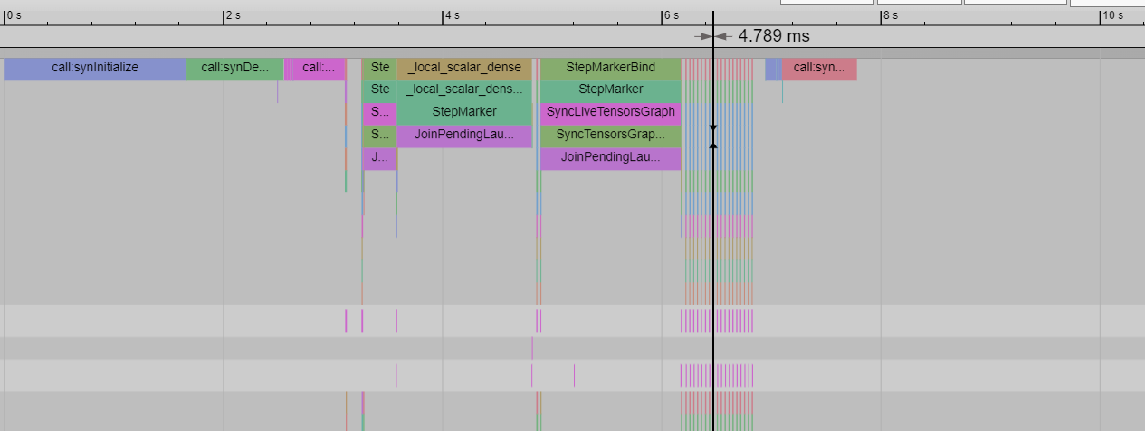
The base case with no HPU Graphs has a CPU processing time of 4.8ms:
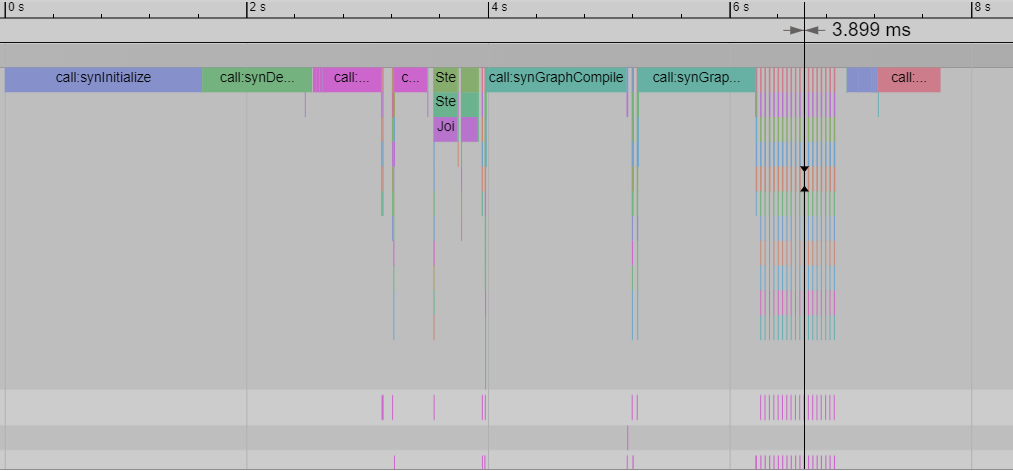
The host profile with make_graphed_callables has a CPU processing time of around 3.9 ms:
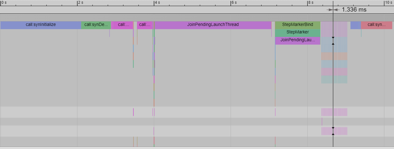
The least host time is observed in the capture and replay mode, with a host time of around 1.3ms:
Next, the effect of each mode on host times is observed. The above modes are run with --steps=20
appended to study the host profile for 20 steps, along with the following environment variables:
PT_FORCED_TRACING_MASK=0xffffffff TRACE_POINT_ENABLE=1 HBN_SYNAPSE_LOGGER_COMMANDS=stop_data_capture:no_eager_flush:use_pid_suffix LD_PRELOAD=/usr/local/lib/python3.8/dist-packages/habana_frameworks/torch/lib/pytorch_synapse_logger.so
The below table shows that make_graphed_callables produces speedup, but capture and replay is the most efficient mode.
Mode |
Time |
|---|---|
No HPU Graphs |
10.937 |
make_graphed_callables |
9.747 |
capture-replay |
6.191 |